Why Sample Variance Divides by (n-1): A Complete Mathematical Proof with Python

Abstract: The sample variance formula uses (n-1) in the denominator rather than n. This article provides a rigorous mathematical proof demonstrating why this "Bessel's correction" makes the sample var

Background: The Bias Problem

When estimating the variance of a population from a sample, we face a subtle but critical problem: we don’t know the true population mean, so we substitute the sample mean. This substitution introduces bias.

Intuition: The sample mean is computed from the same data points we’re using to calculate variance. By construction, it minimizes the sum of squared deviations within that sample. This makes our variance estimate systematically smaller than the true population variance.

Dividing by n (the naive approach) produces a biased estimator. Dividing by (n-1) corrects this bias.

---

What Does “Unbiased” Mean?

An estimator theta_hat is unbiased for a parameter theta if:

\(E[\hat{\theta}] = \theta\)

In our case, we want to show that the expected value of the sample variance equals the population variance:

E[s²] = σ²

If this equality holds, we call s² an unbiased estimator of σ².

---

Setting Up the Proof

Population Variance

The true population variance is defined as:

σ² = E[(X - μ)²]

where μ is the population mean and X represents individual observations.

Sample Variance

The sample variance (with Bessel’s correction) is:

s² = (1/(n-1)) * Σ(x_i - x_bar)²

where x_bar is the sample mean and the sum runs from i=1 to n.

Our goal is to prove:

E[s²] = σ²

---

Core Proof Strategy

We’ll use three key mathematical tools:

1. Linearity of expectation: E[aX + bY] = aE[X] + bE[Y] for constants a, b

2. Expectation of a constant: E[c] = c

3. Known variance identities:

   • Var(X) = E[X²] - (E[X])²

   • Var(x_bar) = σ²/n (variance of the sample mean)

Step 1: Extract the constant from the expectation

Start with:

E[s²] = E[(1/(n-1)) * Σ(x_i - x_bar)²]

By linearity, we can pull the constant (1/(n-1)) outside:

E[s²] = (1/(n-1)) * E[Σ(x_i - x_bar)²]

Step 2: Expand the squared term

Now focus on the summation. Expand the square:

Σ(x_i - x_bar)² = Σ[x_i² - 2x_i*x_bar + x_bar²]

Distribute the sum:

= Σx_i² - 2x_bar*Σx_i + n*x_bar²

Recall that x_bar = (Σx_i)/n, so Σx_i = n*x_bar. Substitute:

= Σx_i² - 2x_bar*(n*x_bar) + n*x_bar²

= Σx_i² - 2n*x_bar² + n*x_bar²

= Σx_i² - n*x_bar²

Step 3: Take expectations

Now apply the expectation operator:

E[Σx_i² - n*x_bar²] = E[Σx_i²] - n*E[x_bar²]

Use the variance identity: Var(X) = E[X²] - (E[X])², which rearranges to E[X²] = Var(X) + (E[X])².

For each x_i:

E[x_i²] = σ² + μ²

So:

E[Σx_i²] = n*(σ² + μ²)

For x_bar:

E[x_bar²] = Var(x_bar) + (E[x_bar])²

= σ²/n + μ²

Substitute these into our equation:

E[Σx_i² - n*x_bar²] = n*(σ² + μ²) - n*(σ²/n + μ²)

= n*σ² + n*μ² - σ² - n*μ²

= n*σ² - σ²

= (n-1)*σ²

Step 4: Combine back with the (1/(n-1)) term

Recall from Step 1:

E[s²] = (1/(n-1)) * E[Σ(x_i - x_bar)²]

Substitute the result from Step 3:

E[s²] = (1/(n-1)) * (n-1)*σ²

E[s²] = σ²

QED. The sample variance s² is an unbiased estimator of the population variance σ².

Why Does This Matter in Practice?

• Hypothesis Testing: T-tests, F-tests, and ANOVA all rely on unbiased variance estimates to construct test statistics with known distributions

• Confidence Intervals: Standard errors (which depend on s) need to be unbiased to produce correct coverage probabilities

• A/B Testing: When computing pooled variance or running two-sample tests, using (n-1) ensures your p-values and confidence intervals are calibrated correctly

• ML Model Evaluation: Bootstrap resampling, cross-validation, and uncertainty quantification all depend on accurate variance estimates

If you used n instead of (n-1), your variance estimates would be systematically too small, leading to:

• Inflated test statistics (more false positives)

• Confidence intervals that are too narrow (overconfidence)

• Underestimated uncertainty in predictions

---

Python Simulation: Seeing the Bias Correction in Action

Let’s empirically demonstrate that dividing by (n-1) produces unbiased estimates, while dividing by n does not.

import numpy as np
import matplotlib.pyplot as plt

# Set random seed for reproducibility
np.random.seed(42)

# True population parameters
population_mean = 50
population_variance = 100  # σ² = 100
population_std = np.sqrt(population_variance)

# Sample sizes to test
sample_size = 30
num_simulations = 10000

# Storage for variance estimates
biased_estimates = []
unbiased_estimates = []

# Run simulations
for _ in range(num_simulations):
    # Draw a random sample from the population
    sample = np.random.normal(population_mean, population_std, sample_size)
    
    # Calculate sample mean
    sample_mean = np.mean(sample)
    
    # Calculate sum of squared deviations
    squared_devs = np.sum((sample - sample_mean)**2)
    
    # Biased estimator (divide by n)
    biased_var = squared_devs / sample_size
    biased_estimates.append(biased_var)
    
    # Unbiased estimator (divide by n-1)
    unbiased_var = squared_devs / (sample_size - 1)
    unbiased_estimates.append(unbiased_var)

# Calculate average of estimates across all simulations
mean_biased = np.mean(biased_estimates)
mean_unbiased = np.mean(unbiased_estimates)

print(f"True population variance: {population_variance}")
print(f"Mean of biased estimates (n): {mean_biased:.4f}")
print(f"Mean of unbiased estimates (n-1): {mean_unbiased:.4f}")
print(f"\nBias with n: {mean_biased - population_variance:.4f}")
print(f"Bias with (n-1): {mean_unbiased - population_variance:.4f}")

Expected Output:

True population variance: 100
Mean of biased estimates (n): 96.5855
Mean of unbiased estimates (n-1): 99.9161

Bias with n: -3.4145
Bias with (n-1): -0.0839

Notice that:

• The biased estimator (dividing by n) consistently underestimates the true variance

• The unbiased estimator (dividing by (n-1)) produces estimates that center around the true value

• Over many simulations, the mean of the unbiased estimates converges to σ² = 100

Visualizing the Distribution of Estimates

# Create histogram comparing both estimators
plt.figure(figsize=(12, 5))

plt.subplot(1, 2, 1)
plt.hist(biased_estimates, bins=50, alpha=0.7, color='red', edgecolor='black')
plt.axvline(population_variance, color='blue', linestyle='--', linewidth=2, label='True σ²')
plt.axvline(mean_biased, color='darkred', linestyle='-', linewidth=2, label='Mean of estimates')
plt.xlabel('Variance Estimate')
plt.ylabel('Frequency')
plt.title('Biased Estimator (divide by n)')
plt.legend()

plt.subplot(1, 2, 2)
plt.hist(unbiased_estimates, bins=50, alpha=0.7, color='green', edgecolor='black')
plt.axvline(population_variance, color='blue', linestyle='--', linewidth=2, label='True σ²')
plt.axvline(mean_unbiased, color='darkgreen', linestyle='-', linewidth=2, label='Mean of estimates')
plt.xlabel('Variance Estimate')
plt.ylabel('Frequency')
plt.title('Unbiased Estimator (divide by n-1)')
plt.legend()

plt.tight_layout()
plt.show()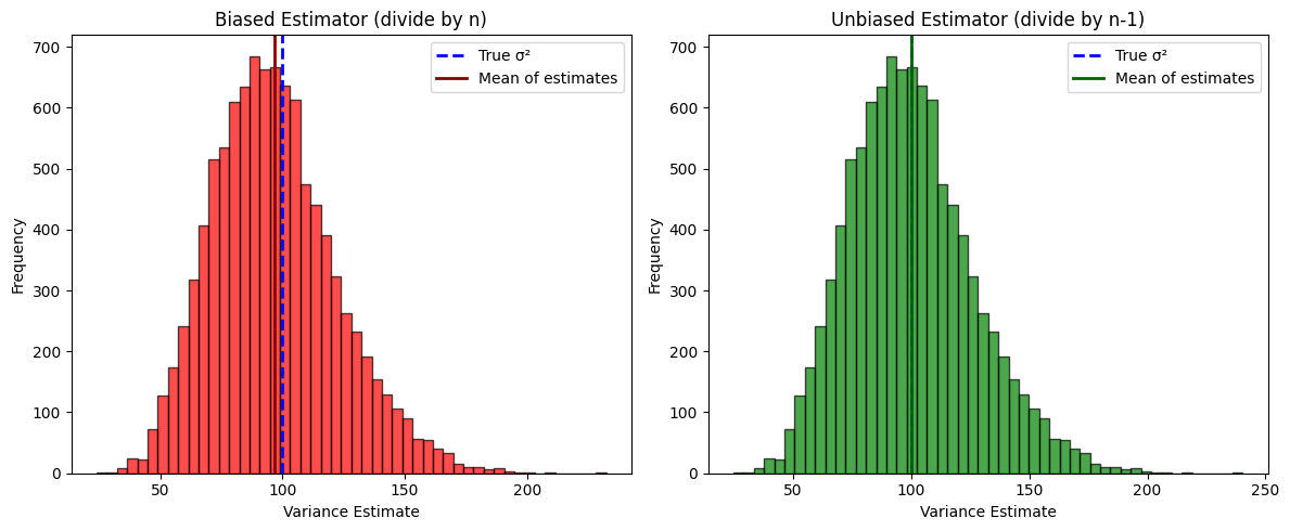

The visualization shows:

• Both estimators produce distributions centered near the true variance

• The biased estimator’s distribution is systematically shifted to the left (underestimation)

• The unbiased estimator’s distribution is properly centered on the true parameter

Common Pitfalls and Practical Tips

Pitfall 1: Confusing standard deviation with variance

• Bessel’s correction applies to variance (s²), not standard deviation (s)

• While s² is unbiased for σ², s is actually slightly biased for σ (though the bias is small for large n)

Pitfall 2: Using the wrong denominator in pandas/numpy

• np.var(data) uses n by default (ddof=0)

• np.var(data, ddof=1) uses (n-1) for unbiased estimation

• pd.Series.var() uses (n-1) by default (ddof=1)

Pitfall 3: Misapplying the correction for population data

• If you have the entire population (not a sample), use n in the denominator

• The correction only applies when estimating from a sample

Tip: Always verify your library’s default behavior for variance calculations, especially when switching between numpy and pandas.

---

Conclusion

The (n-1) denominator in the sample variance formula isn’t arbitrary – it’s a mathematically rigorous correction that ensures our variance estimates are unbiased. This proof demonstrates how the use of the sample mean (instead of the true population mean) systematically reduces the sum of squared deviations, and why dividing by (n-1) exactly compensates for that reduction.

Whether you’re designing experiments, building confidence intervals, or evaluating model uncertainty, understanding this correction helps you avoid subtle statistical errors that can cascade through your analysis pipeline.

Next time you run a t-test or compute a standard error, you’ll know exactly why that (n-1) is there – and why it matters.